Confidence intervals are a standard output of many free and paid A/B testing tools. Most A/B test reports contain one or more interval estimates.
Even if you’re simply a consumer of such reports, understanding confidence intervals is helpful. If you’re in charge of preparing and presenting those reports, it’s essential.
In this article, we’ll look at confidence intervals—what they are, how to interpret them, some caveats, and oft-encountered issues.
What is a confidence interval?
A confidence interval is one way of presenting the uncertainty associated with a given measurement of a parameter of interest.
For example, if we’re interested in the difference between the conversion rate of a test variation of a checkout page and our current checkout page, we would:
- Perform an A/B test to measure the difference between the test and control groups.
- Make a claim regarding the future performance of the test variation versus the current one based on that test.
When communicating the results, it’s a good idea to present not only the observed difference but also a range of values that the data hasn’t ruled out with sufficient certainty. This is where a confidence interval can help.
A confidence interval is a random interval on the real line that, when constructed over repeated tests of the same type with different data, covers the true value of the parameter of interest a specified proportion of the time.
This proportion is the confidence level and is usually expressed as a percentage (e.g., a confidence interval of 90%, 95%, 99%). The term “confidence” is technical and refers specifically to that proportion, which is also referred to as “coverage probability.”
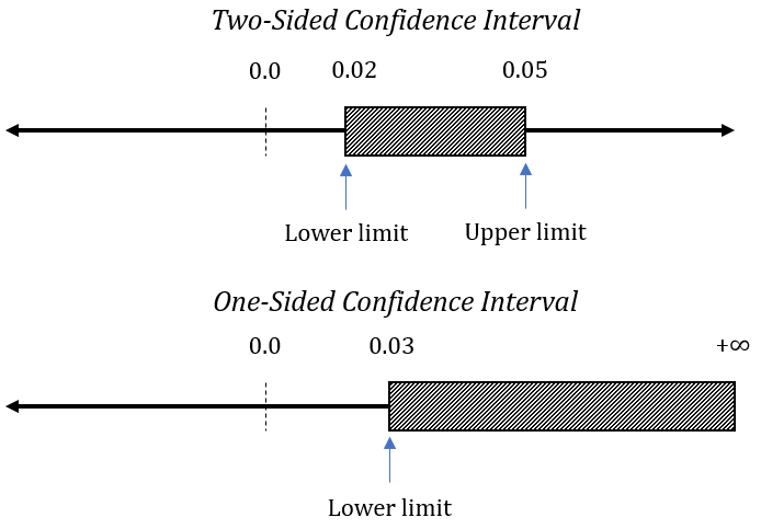
Customarily, confidence intervals are constructed with two bounds—one from above and one from below, also called “confidence limits.” However, an interval can also have a limit on only one side, spanning to minus or plus infinity in the other direction.
While many software packages offer 95% confidence intervals by default (or as the only option), it’s often useful to construct confidence intervals at other levels. Some practitioners even suggest constructing distributions of confidence limits (“confidence distributions”) to explore fully which conclusions the A/B test data warrants.
Before we dig further into the interpretation of these limits and their role in decision-making, let’s look at how they’re constructed.
The mathematical basis of confidence intervals
Many articles on statistical concepts for marketers and UX specialists shy away from presenting formulas. That’s to their detriment: Examining what goes in makes it so much easier to understand what comes out.
Therefore, we’ll start with a bit of math to make the next parts more understandable.
First, the generic formula for calculating the bounds of a confidence interval is:
where
- P is the parameter we are measuring.
- ME is the desired Margin of Error for the parameter, usually based on variability estimates from the data.
In A/B testing, the parameter is usually either the absolute or relative difference in proportions, but it can also be the difference in means of continuous metrics. Most commonly, we work with differences in conversion rates or average revenue per user.
The margin of error is calculated from the estimated standard deviation of the parameter, multiplied by a Z-score corresponding to the chosen confidence level.
For example, the bounds of a confidence interval for the absolute difference between two means are calculated with the following equation:
where
- μ1 is the mean of the baseline or control group.
- μ2 is the mean of the treatment group.
- n1 is the sample size of the baseline or control group.
- n2 is the sample size of the treatment group.
- σp is the pooled standard deviation of the two groups.
- Z is the score statistic corresponding to the desired confidence level.
The formula for the absolute difference of proportions (i.e. conversion rates of all kinds) is the same—they’re just a special type of mean. Examining the formula, we can see why it’s a random interval: The interval bounds depend on:
- The random error introduced by the observed difference in the means;
- The error in estimating the standard deviation of said difference.
Visualized as a distribution of the error of the mean, an interval bound cuts a certain percentage of a distribution centered on the observed value—to the left, to the right, or on both sides.
We can also see that the larger the sample size, the narrower the width of the interval. This happens since we are dividing the pooled standard deviation by a larger number, which ultimately results in a smaller number being added or subtracted from the observed parameter value.
With an infinite sample size, the interval collapses into a single point on the real line. This follows our intuition: The more data we have, the less uncertainty an estimate of the parameter of interest should have.
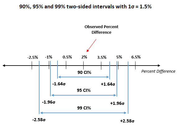
Further, requiring a higher confidence level means a larger value for Z, resulting in a wider interval, and vice versa. A 99% confidence interval will always be wider than a 95% confidence interval, all else being equal.
Note how nothing in the construction of these bounds suggests giving more or less weight to any value within the interval. Each point within the confidence interval is equally likely to be the true value, at least from the standpoint of confidence interval logic.
Interpreting confidence intervals
However simple confidence intervals are, their interpretation can be tricky because they’re a characteristic of the testing procedure, similar to p-values.
A frequent error is to assert that if a calculated 95% confidence interval (derived from test data) includes values such as 0.02 and 0.05, then there is a 95% likelihood that the true value falls within that interval. This confuses the probability of the procedure with the probability of a specific hypothesis (i.e., “the value is between 0.02 and 0.05”).
The mistake is obvious since, for this particular realization of the interval, the true value either is, or is not, within it. For example, if the true value is 0.01, it is outside the current realization of the interval, which spans from 0.02 to 0.05.
When examining the results of an A/B test, the correct way to interpret the outcome in terms of a confidence interval relies on counterfactual reasoning (similar, again, to p-values).
For example, upon observing a 95% interval spanning from 0.02 to 0.05, we can say that claims that the true value lies outside of that interval are not supported by the data. Had the true value been outside of the interval, the statistical procedure would have, with a probability of 95% or greater, returned an interval different than the one observed.
It’s not entirely correct to state that values within the interval are “supported” by the data. The statement of “support” is ambiguous—only one of the values can be the true value, so we cannot claim simultaneous support for all values in the interval. It’s more accurate to say that these values “have not been ruled out.”
In a sense, the values not covered by the interval are what we should focus on, not the values covered by it. What we are often interested in is to make claims like “we can rule out values less than X with 95% confidence,” where X is some minimal value of interest. For example, we may want to implement the tested variant if we can rule out values less than 0.01.
In such cases, it would be incorrect to use the lower bound of a two-sided 95% confidence interval; a one-sided interval should be used instead. Using a two-sided interval to make such a claim overstates the uncertainty.
The 95% two-sided interval would exclude values less than 0.01 with a 97.5% probability if the true value is indeed greater than 0.01. However, a one-sided 95% confidence interval would have a lower limit greater than 0.01 with 95% probability if the true difference is greater than or equal to 0.01, which is exactly what we want.
Finally, as with every statistical estimate, it needs to be based on the parameter of interest. It’s not uncommon to see software plot confidence intervals for the conversion rate of each group in a test. This tempts some users to check the intervals for overlap and judge the outcome based on whether the two intervals overlap.
However, if the difference between the groups is of interest, these intervals are irrelevant. One should instead look at a single interval for the difference in means or proportions. It can easily be shown that the two separate intervals for each group’s metric might overlap, while the interval for the difference between the metrics rules out “no difference.”
Duality with p-values
There’s a one-to-one correspondence between p-values and confidence intervals. They’re based on the same statistical model, and one can usually be easily converted to the other. Consequently, any critiques or praises of p-values apply equally to confidence intervals. Similarly, all prerequisites for proper use of p-values also apply to confidence intervals.
A confidence interval bound defines a set of values, which, if contained as part of the null hypothesis, would not be rejected by the data at a significance threshold corresponding to the interval confidence level. In other words, we would reject any null hypothesis in a Null Hypothesis Statistical Test defined over a set of values, all of which are outside the confidence interval.
For example, if the lower bound of a one-sided 95% interval is -0.01, then H0: Δ ≤ 0 would not be rejected with a p-value less than 0.05, since 0 is greater than -0.01. On the other hand, any H0: Δ ≤ µ0 for µ0 < -0.01 can be rejected.
Converting from a confidence threshold to a significance threshold (p-value threshold) is easy. Simply subtract the confidence threshold from 100% and divide by 100 to get rid of the percentage: 95% confidence level is equivalent to 100% – 95% = 5% / 100 = 0.05 significance threshold.
Confidence intervals for percentage difference
So far, we have used confidence interval examples only for absolute difference. If you want to make claims regarding the relative difference between proportions or means, you need to redefine the statistical model for computing confidence intervals in terms of percentage change (e.g., 1–15%).
Converting from a confidence interval for an absolute difference to one for percentage change shouldn’t be done naively. You can’t simply take the limits for absolute difference and express them as percentages, which results in intervals with incorrect coverage probability.
Since this is a lengthy topic, I would refer you to my blog post on confidence intervals for relative change (i.e. percentage lift).
Conclusion
Confidence intervals are a useful tool for visualizing the uncertainty of data from A/B tests. They help decision-makers assess the risk they’ll take by committing to a certain action.
Their visual nature helps avoid common issues with tools such as p-values; however, many caveats remain.


